From 0 to 30K - The network

“In space, no one can hear you lag” - unless you’re in proximity chat, then everyone hears you rubber-band.

Welcome to the first article in a series exploring computer science concepts through Star Citizen! From network architecture to load balancing, from server coordinates to deadlocks - we’ll be using space mishaps to understand why distributed systems are both fascinating and terrifying. Why Star Citizen? Because explaining distributed systems is hard, but everyone understands the pain of rubber-banding into an asteroid.

Ever wondered why sometimes your perfect shot misses, or why your ship rubber-bands during quantum travel? Let’s start with the network basics behind these daily space dramas. I’ll be using Python to visualize these concepts, because if there’s one thing I love more than filling Hercules with trolleys, it’s turning data into charts.

Fair warning: like CIG’s release dates, all numbers in this article are subject to change and should be taken with enough salt to fill a Starfarer. The goal here isn’t to provide exact figures, but to understand the underlying concepts that make our space shenanigans possible (or occasionally impossible, looking at you, 30k).

All code examples in this article are available in this Python notebook. Feel free to experiment with the numbers - breaking things is how we learn!

Understanding Network Basics #

Before we quantum travel into the deep analysis, let’s understand some key concepts that affect your journey through the verse.

A quick note about the math: in our analysis, we’ll be using two main types of statistical distributions to model network behavior:

• Normal distribution (also called Gaussian) for typical network conditions - think of your regular quantum travel, where most jumps take about the same time with small variations
• Exponential distribution for modeling network issues - like those rare but dramatic moments when your ship decides interpretive dance is its true calling. It gives us lots of normal values but allows for those occasional dramatic spikes

These aren’t just arbitrary choices - they’re commonly used in real network analysis because they match what we actually see in practice. The normal distribution is perfect for modeling stable connections with small variations, while the exponential distribution captures those “rare but significant” events that make space life interesting.

Now, let’s dive into the specific metrics that determine whether your perfect shot lands or your ship decides to cosplay as a pinwheel…

RTT (Round Trip Time) #

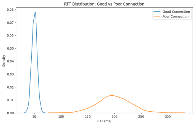
Round Trip Time measures how long it takes for a signal to make a complete journey. In Star Citizen terms:

1. You press the trigger (signal to server)
2. Server processes the shot
3. Server sends back the result
4. Your client shows the hit/miss

# Example from our notebook
import numpy as np
import seaborn as sns
import matplotlib.pyplot as plt

# Simulate RTT measurements
good_connection = np.random.normal(50, 5, 1000)  # Mean 50ms, SD 5ms
poor_connection = np.random.normal(200, 30, 1000)  # Mean 200ms, SD 30ms

# Plot RTT distribution
plt.figure(figsize=(10, 6))
sns.kdeplot(good_connection, label='Good Connection')
sns.kdeplot(poor_connection, label='Poor Connection')
plt.xlabel('RTT (ms)')
plt.title('RTT Distribution: Good vs Poor Connection')
plt.legend()

This directly affects your gameplay:

• Low RTT (~50ms): Your shots feel responsive
• Medium RTT (~150ms): Slight delay but playable
• High RTT (300ms+): Noticeable lag in all actions

RTT isn’t just about your shots landing - it affects everything from cargo trading to mining charge timing. A 300ms delay might be barely noticeable when you’re casually touring Lorville, but it becomes painfully obvious when you’re trying to dodge torpedoes in a dogfight.

That’s why some activities are more “latency sensitive” than others, and why your org mate keeps blaming their “high ping” for losing that 1v1¹.

Jitter: the turbulence² factor #

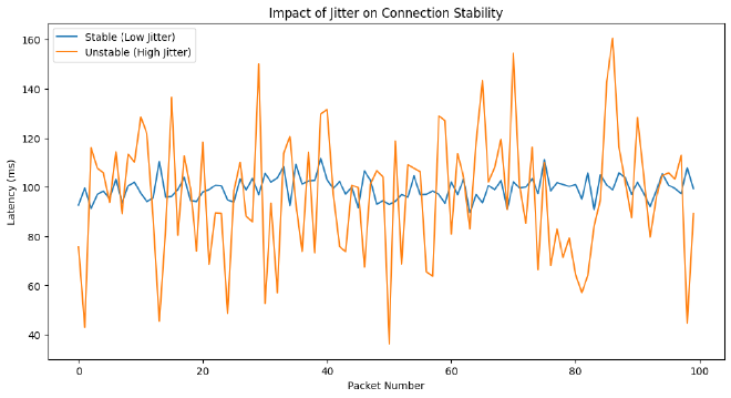
Notice how the “Poor Connection” had a much wider spread than the “Good Connection”? That’s jitter in action. While RTT tells you the average delay, jitter (measured as standard deviation) shows how stable that delay is. It’s like comparing:

• Low jitter (SD ~5ms): Like the tight distribution in our “Good Connection” - smooth quantum travel
• High jitter (SD ~30ms): Like the wide spread in our “Poor Connection” - bumpy atmospheric flight

# Simulate different jitter scenarios
stable = np.random.normal(100, 5, 100)  # Stable connection
unstable = np.random.normal(100, 30, 100)  # Unstable connection

# Plot time series
plt.figure(figsize=(12, 6))
plt.plot(stable, label='Stable (Low Jitter)')
plt.plot(unstable, label='Unstable (High Jitter)')
plt.xlabel('Packet Number')
plt.ylabel('Latency (ms)')
plt.title('Impact of Jitter on Connection Stability')
plt.legend()

This helps explain many common “network weirdness” moments in the verse. High jitter is actually worse for gameplay than consistently high latency - your brain can adapt to a delay, but it can’t adapt to a delay that keeps changing. Think about it: a stable 150ms RTT means you can learn to lead your targets by a consistent amount, but erratic jitter means sometimes you need to lead by 50ms, sometimes by 200ms.

That’s why you might have a higher average ping than your friend but a smoother combat experience - stability often matters more than speed.

Percentiles: beyond the average #

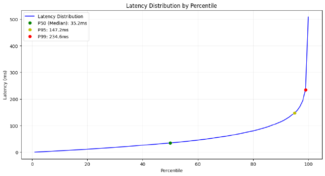
Averages can be misleading. Percentiles give us a better picture:

# Generate realistic game session data
session_data = np.random.exponential(50, 10000)

# Calculate percentiles from 1 to 100
percentiles = range(1, 101)
latencies = np.percentile(session_data, percentiles)

plt.figure(figsize=(12, 6))

# Main plot showing percentiles vs latency
plt.plot(percentiles, latencies, 'b-', label='Latency Distribution')

# Highlight key percentiles
p50 = np.percentile(session_data, 50)
p95 = np.percentile(session_data, 95)
p99 = np.percentile(session_data, 99)

# Add markers for key percentiles
plt.plot(50, p50, 'go', label=f'P50 (Median): {p50:.1f}ms')
plt.plot(95, p95, 'yo', label=f'P95: {p95:.1f}ms')
plt.plot(99, p99, 'ro', label=f'P99: {p99:.1f}ms')

plt.grid(True, alpha=0.2)
plt.xlabel('Percentile')
plt.ylabel('Latency (ms)')
plt.title('Latency Distribution by Percentile')
plt.legend()

Understanding percentiles helps explain those moments when your org mate insists “but my connection is fine!” while their ship is break-dancing across Port Olisar³. Sure, their P50 looks great in discord screenshots, but that P99 tells the real story of why their “perfectly executed landing” ended up redecorating the spaceport.

When it comes to network performance, averages hide the moments that really matter, this helps explain why:

• Your average ping might look fine, but you still experience occasional issues
• Some players have different experiences with similar average connections
• Network problems often feel worse than the numbers suggest

Bandwidth #

“How much bandwidth do you need? Yes.” - CIG Server Engineer, probably

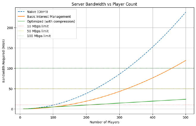
While modern internet connections usually handle client bandwidth needs just fine, it’s worth thinking about the bigger picture. Your client might only need to send and receive data about nearby ships, but imagine being the server:

# Simulate different server bandwidth requirements
def calculate_bandwidth_naive(num_players, data_per_player=1000):  # 1KB per player
    total_bandwidth = 0
    # Each player needs updates about ALL other players
    for player in range(num_players):
        total_bandwidth += (num_players - 1) * data_per_player  # O(n²) scaling
    return total_bandwidth / (1024 * 1024)  # Convert to MB/s

def calculate_bandwidth_basic(num_players, data_per_player=1000):  # 1KB per player
    total_bandwidth = 0
    # Each player needs updates about nearby players
    for player in range(num_players):
        nearby_players = min(num_players - 1, 50)  # Assume max 50 relevant players
        total_bandwidth += nearby_players * data_per_player  # O(n) scaling
    return total_bandwidth / (1024 * 1024)  # Convert to MB/s

def calculate_bandwidth_optimized(num_players, data_per_player=1000):  # 1KB per player
    total_bandwidth = 0
    for player in range(num_players):
        # Use dynamic interest management and compression
        nearby_players = min(num_players - 1, 50)
        compression_ratio = 0.6 + (0.4 * (nearby_players / 50))  # Better compression with fewer players
        total_bandwidth += nearby_players * data_per_player * compression_ratio
    return total_bandwidth / (1024 * 1024)  # Convert to MB/s

players = range(10, 501, 10)
bandwidth_naive = [calculate_bandwidth_naive(n) for n in players]
bandwidth_basic = [calculate_bandwidth_basic(n) for n in players]
bandwidth_optimized = [calculate_bandwidth_optimized(n) for n in players]

plt.figure(figsize=(10, 6))
plt.plot(players, bandwidth_naive, label='Naive (O(n²))', linestyle='--')
plt.plot(players, bandwidth_basic, label='Basic Interest Management')
plt.plot(players, bandwidth_optimized, label='Optimized (with compression)')
plt.title('Server Bandwidth vs Player Count')
plt.xlabel('Number of Players')
plt.ylabel('Bandwidth Required (MB/s)')
plt.legend()
plt.grid(True)

Let’s look at three different approaches to handling server bandwidth:

• Naive approach: Every player gets updates about every other player. This scales quadratically (O(n²)) - imagine the server trying to tell everyone about everyone else’s coffee cups achieving orbit. This is why early MMOs often had strict player caps per server.
• Basic Interest Management: Players only get updates about nearby entities (what Star Citizen calls “bubbles”). While still non-linear, this grows more slowly than the naive approach since each player only tracks a subset of the total population - you don’t need to know about that Reclaimer on the other side of Stanton, but the server load still compounds as player counts increase.
• Optimized Approach: Combines interest management with dynamic compression and optimization. The closer you are to other players, the more detailed the updates need to be. Imagine getting highly detailed info about the ship you’re about to crash into, but just basic position updates for that distant Bengal carrier⁴.

Think about it: every time someone spawns their shiny new 890 Jump (and we know there’s always someone spawning an 890), the server needs to tell everyone nearby about each of its 12,937 polygons and that one coffee cup that’s about to achieve orbit.

So what have we learned this week?⁵ #

Networking isn’t just about having a fast internet connection - it’s a complex dance of RTT, jitter, bandwidth, and percentiles that all work together to determine whether your perfect shot lands or your ship decides to practice interpretive dance during quantum travel.

By analyzing the data and visualizations, we can see why:

• Using averages for network performance is like measuring a quantum drive’s efficiency by counting wake turbulence - technically possible but missing the point
• The P95/P99 metrics explain those “I SWEAR I hit them!” moments better than any conspiracy about CIG’s hit detection
• Your friend’s “perfect” 50ms connection might actually perform worse than your “stable” 100ms one when jitter enters the chat

And perhaps most importantly, we’ve learned that somewhere out there, a server is doing complex bandwidth calculations to figure out how to tell everyone about that one player who decided to fill their C2 with 1E+2 trolleys (because apparently regular notation isn’t enough to express this level of abuse).